
CELLxGENE Census: 5천만 세포 데이터를 API로 조회하기
CELLxGENE Census란?
CELLxGENE Census는 Chan Zuckerberg Initiative(CZI)에서 제공하는 단일세포 데이터 플랫폼입니다. 전 세계 연구자들이 공개한 5천만 개 이상의 세포 데이터를 하나의 Python SDK로 쿼리할 수 있습니다.
일반적으로 scRNA-seq 데이터를 얻으려면 GEO에서 데이터셋을 찾고, 다운로드하고, 포맷을 맞추고, 통합해야 합니다. Census는 이 과정을 한 줄의 쿼리로 대체합니다.
뭘 조회할 수 있나
Census의 핵심은 필터 기반 쿼리입니다. 원하는 조건을 조합해서 데이터를 가져옵니다:
| 필터 | 예시 |
|---|---|
| cell_type | T cell, B cell, macrophage, hepatocyte, neuron |
| tissue | lung, liver, brain, blood, kidney |
| disease | normal, lung adenocarcinoma, glioblastoma |
| sex | male, female |
| organism | Homo sapiens, Mus musculus |
이 필터들을 조합하면 매우 구체적인 쿼리가 가능합니다:
- “인간 폐의 T cell에서 CD3E 발현”
- “간암 vs 정상 간의 macrophage 비교”
- “삼중음성 유방암의 B cell 유전자 발현 패턴”
암종 데이터
Census에는 다양한 암종 데이터가 포함되어 있습니다. CELLxGENE API로 실제 확인한 데이터 규모:
| 암종 | 데이터셋 수 | 세포 수 |
|---|---|---|
| Lung adenocarcinoma | 12 | 4,939,955 |
| Squamous cell lung carcinoma | 4 | 4,494,669 |
| Glioblastoma | 6 | 1,830,729 |
| B-cell non-Hodgkin lymphoma | 6 | 1,590,877 |
| Malignant ovarian serous tumor | 5 | 1,549,547 |
| Breast cancer | 34 | 1,308,712 |
| Melanoma | 2 | 747,904 |
| Renal cell carcinoma | 20 | 745,504 |
| Neuroblastoma | 3 | 592,116 |
| Basal cell carcinoma | 11 | 557,907 |
| Triple-negative breast carcinoma | 16 | 544,075 |
폐선암만 해도 490만 세포, 유방암 전체는 130만 세포 규모입니다.
설치 및 기본 사용법
설치
pip install cellxgene-census
Windows에서는 tiledbsoma 빌드가 안 됩니다. Linux/macOS를 사용하거나 WSL, Docker, Google Colab에서 실행하세요. Colab이 가장 간편합니다.
기본 구조
import cellxgene_census

with cellxgene_census.open_soma() as census:
    # census['census_data']['homo_sapiens']  → 인간 데이터
    # census['census_data']['mus_musculus']  → 마우스 데이터

    adata = cellxgene_census.get_anndata(
        census,
        organism="Homo sapiens",
        obs_value_filter="...",   # 세포 필터
        var_value_filter="...",   # 유전자 필터
    )
get_anndata()가 핵심 함수입니다. 조건에 맞는 세포만 AnnData 객체로 반환합니다.
실습 예시
1) 정상 폐 T cell의 marker 유전자 발현
import cellxgene_census

with cellxgene_census.open_soma(census_version="2025-11-08") as census:
    adata = cellxgene_census.get_anndata(
        census,
        organism="Homo sapiens",
        obs_value_filter=(
            "tissue_general == 'lung' "
            "and cell_type == 'T cell' "
            "and disease == 'normal'"
        ),
        var_value_filter="feature_name in ['CD3E', 'CD4', 'CD8A', 'FOXP3', 'IL2RA']",
    )

    print(f"세포 수: {adata.n_obs}")
    print(f"유전자: {list(adata.var['feature_name'])}")
    print(f"평균 발현:\n{adata.to_df().mean()}")
아래는 Census 2025-11-08 스냅샷 기준 실제 실행 결과입니다:
세포 수: 78,737
유전자: ['CD8A', 'CD3E', 'CD4', 'FOXP3', 'IL2RA']
평균 발현:
feature_name
CD8A     0.9441
CD3E     1.4457
CD4      0.2718
FOXP3    0.0213
IL2RA    0.0947
78,737개 정상 폐 T cell에서 CD3E(pan-T marker)가 가장 높고, CD8A > CD4 순입니다. FOXP3(Treg marker)는 매우 낮아 Treg 비율이 적음을 시사합니다.
2) 폐선암 vs 정상 폐 — Macrophage 비교
import cellxgene_census

with cellxgene_census.open_soma(census_version="2025-11-08") as census:
    # 폐선암 macrophage
    tumor = cellxgene_census.get_anndata(
        census,
        organism="Homo sapiens",
        obs_value_filter=(
            "tissue_general == 'lung' "
            "and cell_type == 'macrophage' "
            "and disease == 'lung adenocarcinoma'"
        ),
        var_value_filter="feature_name in ['CD68', 'CD163', 'MRC1', 'CD274', 'TGFB1']",
    )

    # 정상 폐 macrophage
    normal = cellxgene_census.get_anndata(
        census,
        organism="Homo sapiens",
        obs_value_filter=(
            "tissue_general == 'lung' "
            "and cell_type == 'macrophage' "
            "and disease == 'normal'"
        ),
        var_value_filter="feature_name in ['CD68', 'CD163', 'MRC1', 'CD274', 'TGFB1']",
    )

    print(f"Tumor macrophages: {tumor.n_obs} cells")
    print(f"Normal macrophages: {normal.n_obs} cells")
    print(f"\n--- Mean expression ---")
    print(f"Tumor:\n{tumor.to_df().mean()}")
    print(f"\nNormal:\n{normal.to_df().mean()}")
실제 실행 결과:
Tumor macrophages: 84,820 cells
Normal macrophages: 534,131 cells

--- Mean expression ---
Tumor:
feature_name
MRC1     10.3532
CD163     7.9206
CD68     26.8582
TGFB1     0.8132
CD274     0.4109

Normal:
feature_name
MRC1     14.5738
CD163    16.0036
CD68     15.5566
TGFB1     2.2421
CD274     0.1283
CD274(PD-L1)가 종양 macrophage에서 약 3.2배 높습니다 (0.41 vs 0.13). 종양 미세환경에서 macrophage가 PD-L1을 통한 면역 억제에 관여함을 시사합니다. 또한 CD68이 종양에서 크게 상승(26.9 vs 15.6)한 반면, CD163과 MRC1(M2 marker)은 정상에서 더 높아, 종양과 정상 macrophage의 표현형 차이를 보여줍니다.
3) 폐선암 세포 유형 구성 (실제 실행 결과)
발현 데이터 없이 메타데이터만 조회할 때는 get_obs()를 사용합니다. 훨씬 가볍고 빠릅니다.
import cellxgene_census

with cellxgene_census.open_soma(census_version="2025-11-08") as census:
    obs_df = cellxgene_census.get_obs(
        census,
        organism="Homo sapiens",
        value_filter="tissue_general == 'lung' and disease == 'lung adenocarcinoma'",
        column_names=["cell_type", "disease", "tissue"],
    )

    print(f"총 세포 수: {len(obs_df)}")
    print(obs_df['cell_type'].value_counts().head(15))
아래는 WSL Ubuntu 환경에서 실제 실행한 결과입니다:
총 세포 수: 1,190,858

cell_type
CD4-positive, alpha-beta T cell         166,387
CD8-positive, alpha-beta T cell         147,701
alveolar macrophage                     102,988
macrophage                               84,820
T cell                                   82,143
natural killer cell                      63,985
B cell                                   62,351
malignant cell                           56,502
classical monocyte                       43,371
epithelial cell of lung                  33,765
regulatory T cell                        31,818
epithelial cell                          29,519
CD1c-positive myeloid dendritic cell     28,159
plasma cell                              26,996
pulmonary alveolar type 2 cell           22,679
119만 세포에서 세포 유형별 구성을 확인할 수 있습니다. CD4+ T cell과 CD8+ T cell이 가장 많고, macrophage(alveolar + general)가 약 18만으로 종양 미세환경에서 큰 비중을 차지합니다.
4) Glioblastoma — 종양 미세환경 유전자 발현
Census에서 GBM의 T cell은 'T cell'이 아닌 'mature T cell'로 annotation되어 있으므로 주의가 필요합니다.
import cellxgene_census
import pandas as pd

with cellxgene_census.open_soma(census_version="2025-11-08") as census:
    adata = cellxgene_census.get_anndata(
        census,
        organism="Homo sapiens",
        obs_value_filter=(
            "disease == 'glioblastoma' "
            "and (cell_type == 'mature T cell' "
            "or cell_type == 'macrophage' "
            "or cell_type == 'microglial cell')"
        ),
        var_value_filter=(
            "feature_name in ['PDCD1', 'CD274', 'CTLA4', 'HAVCR2', "
            "'LAG3', 'TIGIT', 'CD68', 'TMEM119']"
        ),
    )

    print(f"세포 수: {adata.n_obs}")

    # 세포 유형별 평균 발현
    expr = adata.to_df()
    expr['cell_type'] = adata.obs['cell_type'].values
    print(expr.groupby('cell_type', observed=True).mean())
실제 실행 결과:
세포 수: 872,539

세포 유형별 평균 발현:
feature_name     HAVCR2  TMEM119   CD68   LAG3  CD274  CTLA4  TIGIT  PDCD1
cell_type
macrophage       4.6546   0.9814  8.7491 0.0525 0.0766 0.0429 0.0152 0.0776
mature T cell    0.2782   0.0209  0.1399 0.5523 0.0577 0.5051 0.5633 0.4437
microglial cell  3.6666   1.3560  5.0900 0.0283 0.1629 0.0223 0.0089 0.0427

세포 유형별 세포 수:
macrophage         411,937
microglial cell    304,400
mature T cell      156,202
87만 세포 규모의 GBM 면역 미세환경 분석 결과입니다. T cell에서는 면역 checkpoint인 TIGIT(0.56), CTLA4(0.51), LAG3(0.55), PDCD1/PD-1(0.44)이 높게 발현되어 T cell exhaustion을 시사합니다. 반면 macrophage와 microglia에서는 HAVCR2(TIM-3)와 CD68이 지배적이고, microglia에서는 TMEM119이 다른 세포 유형(macrophage 0.98, mature T cell 0.02)에 비해 가장 높게 발현(1.36)되어 microglia-specific marker임을 확인할 수 있습니다.
5) Spatial Transcriptomics 데이터 조회
Census 2025-01-30 스냅샷부터 Spatial Transcriptomics 데이터가 베타로 포함되었습니다. scRNA-seq과 별도로 census_spatial_sequencing 컬렉션에 저장되어 있습니다.
import cellxgene_census
import tiledbsoma

with cellxgene_census.open_soma(census_version="2025-01-30") as census:
    exp = census["census_spatial_sequencing"]["homo_sapiens"]

    cell_metadata = exp.obs.read(
        column_names=["assay", "cell_type", "tissue_general", "disease"]
    ).concat().to_pandas()

    print(f"Total spatial cells: {len(cell_metadata)}")
    print(f"\nAssays:\n{cell_metadata['assay'].value_counts()}")
    print(f"\nTissues:\n{cell_metadata['tissue_general'].value_counts().head(10)}")
    print(f"\nDiseases:\n{cell_metadata['disease'].value_counts().head(5)}")
실제 실행 결과:
Total spatial cells: 2,967,531

Assays:
Slide-seqV2                       1,634,667
Visium Spatial Gene Expression    1,332,864

Tissues:
kidney             1,037,593
heart                362,184
lung                 275,274
lymph node           246,056
liver                158,148
endocrine gland      154,752
skin of body         124,800
exocrine gland       119,808
breast                90,697
colon                 69,888

Diseases:
normal                              1,896,909
renal cell carcinoma                  238,027
metastatic melanoma                   220,029
breast cancer                         184,693
myocardial infarction                 119,808
약 297만 spot/cell의 spatial 데이터가 포함되어 있으며, Visium과 Slide-seqV2 두 가지 assay를 지원합니다. kidney, heart, lung 등 다양한 조직이 포함되어 있습니다.
주의: Spatial 데이터는 일반
census_data가 아닌census_spatial_sequencing컬렉션에 있습니다. 접근 방식이 다르므로get_anndata()/get_obs()대신exp.obs.read()를 사용합니다.
SpatialData 포맷으로 변환
spatial 좌표까지 포함한 분석을 하려면 SpatialData 포맷으로 변환합니다. tiledbsoma>=1.15.3과 spatialdata 패키지가 필요합니다.
import cellxgene_census
import tiledbsoma

census = cellxgene_census.open_soma(census_version="2025-01-30")
exp = census["census_spatial_sequencing"]["homo_sapiens"]

with exp.axis_query(
    measurement_name="RNA",
    obs_query=tiledbsoma.AxisQuery(
        value_filter="tissue_general == 'kidney' and assay == 'Visium Spatial Gene Expression'"
    )
) as query:
    sdata = query.to_spatialdata(X_name="raw")

print(sdata)
census.close()
실제 실행 결과:
SpatialData object
├── Images
│     ├── '05f813a4-..._GRCh38-2020-A': DataArray[cyx] (3, 1834, 2000)
│     ├── '0671c0d4-..._GRCh38-2020-A': DataArray[cyx] (3, 2000, 2000)
│     └── ... (16개 H&E 이미지)
├── Shapes
│     ├── '05f813a4-..._loc': GeoDataFrame shape: (4,992, 3) (2D shapes)
│     ├── '0671c0d4-..._loc': GeoDataFrame shape: (4,992, 3) (2D shapes)
│     └── ... (16개 슬라이드 좌표)
└── Tables
      └── 'RNA': AnnData (79,872, 44,405)
16개 Visium 슬라이드에서 79,872 spots x 44,405 genes의 발현 데이터와 함께 H&E 이미지, 공간 좌표가 포함됩니다.
Shapes에는 각 spot의 좌표가 POINT(x, y) 형태로 저장되어 있습니다:
   soma_joinid     radius           geometry
0      2264134  36.750596  POINT (1422 1194)
1      2264010  36.750596  POINT (1422 1390)
2      2265857  36.750596  POINT (1422 1587)
변환된 SpatialData에는 H&E 이미지, 공간 좌표, 발현 데이터가 모두 포함되어 있어, 조직 구조 위에 직접 시각화할 수 있습니다. 아래는 하나의 kidney Visium 슬라이드(4,992 spots)의 H&E overlay 결과입니다.
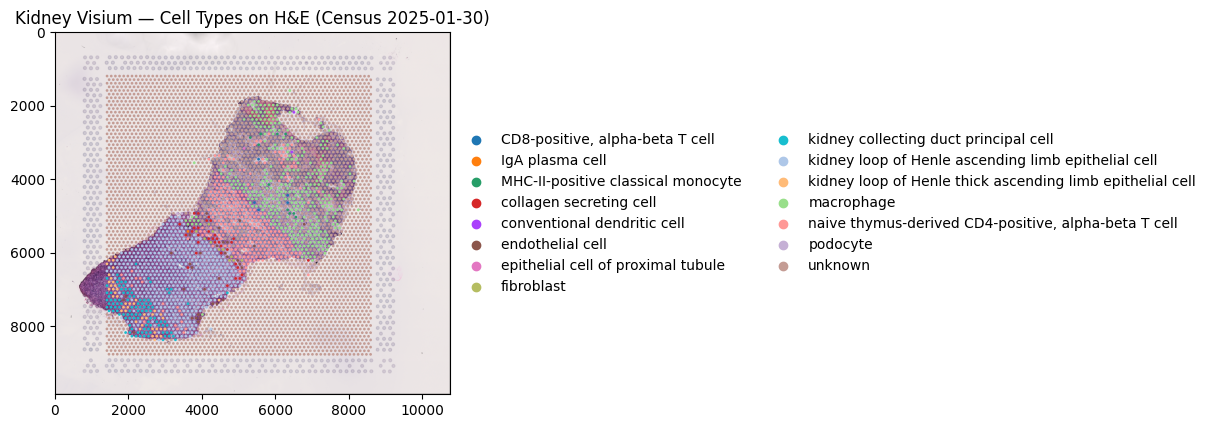
H&E 조직 이미지 위에 세포 유형을 오버레이한 결과입니다. Loop of Henle 상피세포(파란색), macrophage(주황색), CD4+ T cell(초록색) 등이 조직 영역 내에 분포하고 있습니다. 전체 4,992 spots 중 약 70%(3,487개)가 unknown으로, 이는 Visium의 ~55μm spot 해상도 한계로 여러 세포가 하나의 spot에 섞여 명확한 세포 유형 할당이 어렵기 때문입니다. 보다 정밀한 분석을 위해서는 cell2location 같은 deconvolution 방법이 필요합니다.
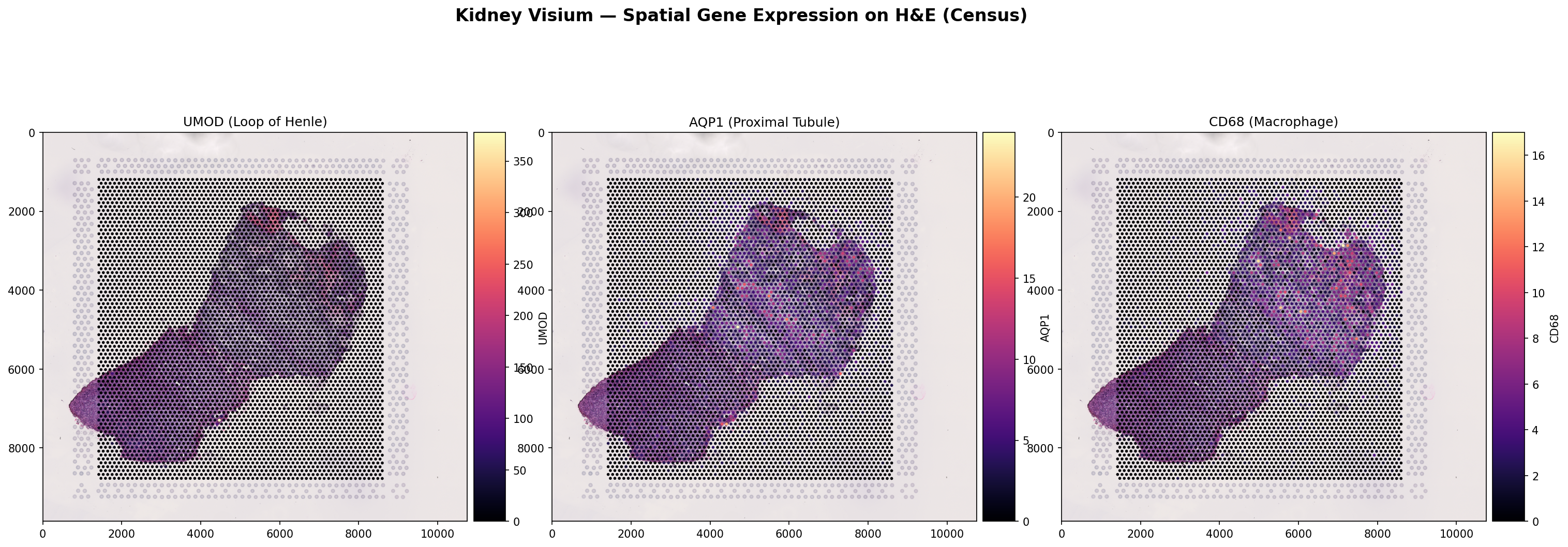
H&E 이미지 위에 유전자 발현(log1p)을 오버레이한 결과입니다. UMOD(Loop of Henle marker, 1,917 spots), AQP1(Proximal Tubule, 2,677 spots), CD68(Macrophage, 1,998 spots)의 발현 분포를 조직 구조와 함께 확인할 수 있습니다. 이 해상도에서는 피질/수질 경계가 명확히 드러나지 않지만, 각 marker의 발현 강도 차이는 관찰됩니다.
MCP Tool로 만들기
이전 AlphaGenome 포스트와 마찬가지로, Census SDK를 MCP Tool로 감싸면 자연어로 쿼리할 수 있습니다.
# cellxgene_mcp.py
from mcp.server.fastmcp import FastMCP
import cellxgene_census

mcp = FastMCP("cellxgene")

@mcp.tool()
def query_expression(
    tissue: str,
    cell_type: str,
    genes: list[str],
    disease: str = "normal",
    organism: str = "Homo sapiens",
) -> dict:
    """특정 조직/세포 유형의 유전자 발현을 조회합니다."""

    gene_filter = ", ".join([f"'{g}'" for g in genes])

    with cellxgene_census.open_soma() as census:
        adata = cellxgene_census.get_anndata(
            census,
            organism=organism,
            obs_value_filter=(
                f"tissue_general == '{tissue}' "
                f"and cell_type == '{cell_type}' "
                f"and disease == '{disease}'"
            ),
            var_value_filter=f"feature_name in [{gene_filter}]",
        )

    expr_mean = adata.to_df().mean().to_dict()

    return {
        "tissue": tissue,
        "cell_type": cell_type,
        "disease": disease,
        "n_cells": adata.n_obs,
        "genes": {g: round(v, 4) for g, v in expr_mean.items()},
    }


@mcp.tool()
def query_cell_composition(
    disease: str,
    organism: str = "Homo sapiens",
) -> dict:
    """특정 질병의 세포 유형 구성을 조회합니다."""

    with cellxgene_census.open_soma() as census:
        obs_df = cellxgene_census.get_obs(
            census,
            organism=organism,
            value_filter=f"disease == '{disease}'",
            column_names=["cell_type"],
        )

    counts = obs_df['cell_type'].value_counts().head(10).to_dict()

    return {
        "disease": disease,
        "total_cells": len(obs_df),
        "top_cell_types": counts,
    }

if __name__ == "__main__":
    mcp.run()
사용 예시
사용자: "폐선암의 T cell과 macrophage에서 PD-L1(CD274) 발현을 비교해줘"

Claude: cellxgene query_expression 도구를 2번 호출하겠습니다.

1) T cell, lung, lung adenocarcinoma, CD274
   → 82,143 cells, CD274 평균 발현: 0.0144

2) macrophage, lung, lung adenocarcinoma, CD274
   → 84,820 cells, CD274 평균 발현: 0.4109

macrophage에서 PD-L1 발현이 T cell 대비 약 28.5배 높습니다.
종양 미세환경에서 macrophage가 PD-L1을 통한 면역 억제에
주요 역할을 하고 있음을 시사합니다.
AlphaGenome과 조합하기
Census와 AlphaGenome을 함께 쓰면 더 강력합니다:
1. CELLxGENE Census로 특정 암종의 DEG(차등발현유전자) 확인
2. DEG 중 regulatory variant가 있는 유전자 선별
3. AlphaGenome으로 해당 variant의 기능적 영향 예측
예: “GBM에서 과발현되는 유전자 중 known variant의 splicing 영향 분석”
논문 한 편 분량의 분석을 MCP Tool 몇 번 호출로 수행할 수 있습니다.
제한사항
| 항목 | 내용 |
|---|---|
| 설치 | Linux/macOS 권장, Windows는 WSL 필요 |
| 데이터 크기 | 전체 다운로드 시 수백 GB, 쿼리 기반 접근 권장 |
| 업데이트 | Census는 주기적으로 스냅샷 업데이트 (최신 데이터셋 반영에 지연) |
| 정규화 | raw count 기반, 정규화는 사용자가 직접 수행 |
| 비용 | 무료 |
마무리
CELLxGENE Census는 scRNA-seq 분야에서 유일하게 API로 접근 가능한 대규모 데이터 플랫폼입니다. GEO에서 데이터셋을 하나씩 다운로드하던 시대와 비교하면, “폐선암 macrophage의 PD-L1 발현”을 코드 한 줄로 조회할 수 있다는 건 엄청난 변화입니다.
여기에 MCP Tool로 감싸면 자연어로 쿼리하고, AlphaGenome과 조합하면 변이 기능 예측까지 이어지는 파이프라인을 구성할 수 있습니다.

댓글남기기