
Hail - (5) Matrix Table
Matrix Table
Matrix Table은 처음 게시글에서 설명했듯이 유전정보를 담고 있는 데이터를 효율적으로 다루기 위해 설계된 Dataframe입니다. 총 4개의 field groups(Entry, Row, Column, Global fields)로 구성되어 있고, Hail Table과 마찬가지로 병렬처리를 위해 partition으로 Table이 나누어져 있습니다. 저번에 다뤘던 Hail Table과 마찬가지로 예제를 통해 읽는 방법부터 시작하여 변환하고 쓰는 방법까지 알려드리려고 합니다. 예제 파일은 Hail Tutorial에서 사용되는 1000 Genomes dataset의 일부입니다.
hl.utils.get_1kg('data/')
다음 코드를 이용하여 VCF 파일과 샘플의 정보를 담고 있는 텍스트 파일들을 Hail로부터 직접 다운받을 수 있습니다. Matrix Table을 생성하는 것부터 차례대로 해볼까요?
1) 읽기 (Read & Import)
Genomics 데이터를 다루는 사람이라면 샘플의 Variant Call 정보를 담고 있는 VCF나, PLINK, BGEN과 같은 여러 형식의 파일을 마주하게 됩니다. 물론 행렬 형식으로 구성된 텍스트 파일을 통해서 Matrix Table을 만들 수 있지만, 일반적으로 다음과 같은 형식의 파일을 Matrix Table로 바꿔주는 함수를 더 많이 사용하게 될 것입니다. 예를 들어, 예제 파일 중 1kg.vcf.bgz은 import_vcf 함수를 사용하면 됩니다.
hl.import_vcf('data/1kg.vcf.bgz').write('data/1kg.mt', overwrite=True)
여기서 한가지 tip이 있다면 VCF 파일을 import했다면 연산을 하기 전에 Matrix Table로 저장을 해두는 것입니다. 그 이유는 Hail의 연산 특징 때문인데요, 이전에 했던 연산을 이미 거쳤더라도 연산의 결과를 저장하지 않으면 연산 과정을 반복하는 경우가 있습니다. 예를 들어, VCF를 (1)Matrix Table로 변환하고 (2)MAF(Minor Allele Frequency)가 5% 이상인 common variants를 선별하고 (3)variants의 수를 확인한다고 했을 때 (1) -> (2) -> (3)의 연산이 차례대로 실행될 것입니다. 그 다음에 (4)variants의 DP 분포를 histogram으로 나타냈다고 하면 (4)번 연산만 실행된다고 생각하지만 실제로는 (1) -> (2) -> (4), 즉 (1), (2)이 반복되어 실행이 됩니다. 보통 import에 쓰이는 함수는 시간이 오래 걸리는 편이므로 import하고 바로 저장을 하여 (1) 과정이 반복되지 않게 해주면 시간 절약이 됩니다. 위의 코드의 경우 write 함수를 통해서 Matrix Table을 바로 저장하였습니다.
import_vcf 함수를 사용하여 VCF를 변환할 때 가끔 애먹는 경우가 있는데, 가령 VCF의 Reference Genome이 GRCh38임에도 불구하고 염색체 이름이 GRCh37의 형식으로 되어 있는 경우가 있습니다. 이 때는 contig_recoding parameter를 이용하여 다음과 같이 import를 해주면 되겠습니다.
recode = {f"{i}":f"chr{i}" for i in (list(range(1, 23)) + ['X', 'Y'])}
ds = hl.import_vcf('data/grch38_bad_contig_names.vcf',
                   reference_genome='GRCh38',
                   contig_recoding=recode)
그 이외에 Reference Genome에는 존재하지 않는 loci가 존재하는 경우 skip_invalid_loci=True 설정을 이용하여 제거해주는 방법도 있습니다.
----------------------------------------
Global fields:
    None
----------------------------------------
Column fields:
    's': str
----------------------------------------
Row fields:
    'locus': locus<GRCh37>
    'alleles': array<str>
    'rsid': str
    'qual': float64
    'filters': set<str>
    'info': struct {
        AC: array<int32>,
        AF: array<float64>,
        AN: int32,
        BaseQRankSum: float64,
        ClippingRankSum: float64,
        DP: int32,
        DS: bool,
        FS: float64,
        HaplotypeScore: float64,
        InbreedingCoeff: float64,
        MLEAC: array<int32>,
        MLEAF: array<float64>,
        MQ: float64,
        MQ0: int32,
        MQRankSum: float64,
        QD: float64,
        ReadPosRankSum: float64,
        set: str
    }
----------------------------------------
Entry fields:
    'GT': call
    'AD': array<int32>
    'DP': int32
    'GQ': int32
    'PL': array<int32>
----------------------------------------
Column key: ['s']
Row key: ['locus', 'alleles']
----------------------------------------
mt의 schema는 다음과 같습니다. 이제 여러가지 함수들을 소개할텐데 이 함수들에 의해 schema가 어떻게 바뀌는지를 주목하며 글을 읽어주시면 좋을 것 같습니다.
2) Row, Column, Entry Table 추출
Matrix Table 자체는 데이터의 양이 매우 크기 때문에 우리가 Row fields 또는 Column fields만 작업에 사용할 예정이라면, 그 Table을 추출하여 효율적인 작업을 할 수 있을 것입니다. Matrix Table의 Row Table 또는 Column Table을 추출하는 방법은 rows, cols 함수를 이용하면 됩니다. 예를 들어 mt의 Row Table을 추출하고 schema를 확인하면 다음과 같습니다.
mt.rows().describe()
----------------------------------------
Global fields:
    None
----------------------------------------
Row fields:
    'locus': locus<GRCh37>
    'alleles': array<str>
    'rsid': str
    'qual': float64
    'filters': set<str>
    'info': struct {
        AC: array<int32>,
        AF: array<float64>,
        AN: int32,
        BaseQRankSum: float64,
        ClippingRankSum: float64,
        DP: int32,
        DS: bool,
        FS: float64,
        HaplotypeScore: float64,
        InbreedingCoeff: float64,
        MLEAC: array<int32>,
        MLEAF: array<float64>,
        MQ: float64,
        MQ0: int32,
        MQRankSum: float64,
        QD: float64,
        ReadPosRankSum: float64,
        set: str
    }
----------------------------------------
Key: ['locus', 'alleles']
----------------------------------------
위의 경우 Column, Entry fields는 없고 Row fields만 있는 Table을 얻는 것을 확인할 수 있습니다. 또한 우리가 matrix 형태로 되어 있는 Entry fields를 Row key와 Column key를 key로 하는 Table 형태로 얻고 싶다고 할 때 entries 함수를 사용할 수 있습니다. 이 때 주의해야 할 것은 Entry Table의 메모리 문제입니다. Matrix Table이 N개의 행, M개의 열로 이루어져 있다고 하면 entries 함수로 추출된 Table의 행의 개수는 N*M개나 됩니다. Hail Docs에서 설명하길 Matrix Table을 Entry Table로 바꾸게 되면 기존 저장공간의 100배 이상을 쓰게 된다고 합니다. 따라서 Row field와 Column field를 동시에 grouping하여 aggregation하는 것과 같은 특수한 경우를 빼면 Matrix Table이 클수록 Entry Table로 바꾸는 것은 주의하여야 할 것입니다.
3) Filtering
보통 Genomics 데이터 분석을 하기 전에 전처리 과정으로 QC(Quality Control)를 하게 되는데요, VCF 파일의 경우 보통 FILTER field, INFO field(QD, MQ 등), 그리고 샘플마다 Format field로 정의된 값(GT, DP 등)을 기준으로 유전변이를 분석에 포함할지를 결정하게 됩니다. FILTER field의 경우 기준을 통과하면 PASS, 그렇지 않으면 만족하지 못한 기준이 표시가 되는데, GATK에서 VQSR한 경우를 예로 들면 VQSRTrancheSNP99.00to99.90+와 같은 형태로 표시가 됩니다. Matrix Table에서는 FILTER field가 filters라는 field로 대체되고 data type이 SetExpression으로 되어 있어 있습니다. (e.g. {"VQSRTrancheSNP99.00to99.90+"}) 주의할 점은 편의를 위해 기준을 전부 통과한 유전변이의 경우에는 PASS가 아닌 {}로 표시되어 있어서 기준을 통과한 유전변이를 subset하고 싶다면 다음과 같이 코드를 작성하면 됩니다.
mt = mt.filter_rows(hl.len(mt.filters) == 0)
Row, Column, Entry field마다 filter를 적용하는 함수가 각각 filter_rows, filter_cols, filter_entries로 다르기 때문에 주의해야 합니다. 예를 들어, INFO field의 quality metrics를 통해 filtering을 하고 싶다면 filter_rows, Entry field에 있는 각 샘플의 quality metrics를 이용하여 filtering을 하려면 filter_entries를 사용합니다. 그렇다면 예제를 이용하여 AF가 5% 미만인 유전변이와 GQ가 25보다 적은 call을 제외하는 코드를 살펴보고 plot도 한번 그려보겠습니다. 우선 plot을 그리는 데에 필요한 패키지를 불러옵시다.
from bokeh.io import show, output_notebook
from bokeh.layouts import gridplot
output_notebook()
Hail은 bokeh 패키지를 plot 그리는 데에 사용하는데 여기서 output_notebook 함수는 jupyter notebook에서 cell 실행 결과로 plot를 출력한다는 설정입니다. 다음은 두 기준에 대해서 filter를 적용하고 plotting하는 코드입니다.
mt = mt.filter_rows(mt.info.AF[0] > 0.05)
p1 = hl.plot.histogram(mt.info.AF[0], range=(0,1), title='MAF')

mt = mt.filter_entries(mt.GQ >= 25)
p2 = hl.plot.histogram(mt.GQ, range=(0, 100), title='GQ')

show(gridplot([p1, p2], ncols=2, plot_width=400, plot_height=400))
코드와 관련해서 도움이 될 만한 정보를 몇 가지 알려드리러 합니다. mt.describe() 코드를 실행하면 18개의 fields를 포함하는 info field를 확인할 수 있을 것입니다. 이 형태를 Hail에서는 Struct라고 하는데, fields 간의 관계를 체계화하기 좋은 data type입니다. Struct 안의 field에 접근하는 방법은 Table에서 하는 것과 마찬가지로 [, ] 또는 .을 이용합니다. 예를 들어, mt의 info 안에 AF field에 접근하고 싶다고 하면 mt.info.AF 또는 mt['info']['AF']와 같은 방법을 사용할 수 있습니다.
histogram 함수를 이용하면 내가 확인하고자 하는 metric의 분포를 바로 확인할 수 있어서 편리합니다. range parameter를 통해 histogram 축의 범위를 설정해주었습니다. 각각의 histogram을 p1, p2로 정의하고 gridplot을 이용하여 두 그래프을 한꺼번에 나타내려고 합니다.
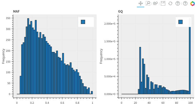
그래프는 다음과 같이 그려지는데요, 첫번째 그래프의 경우에 AF 값이 5% 밑으로 존재하지 않음을 확인할 수 있고 두번째 그래프는 GQ 값이 25 밑의 값이 존재하지 않음을 확인할 수 있습니다.
4) Adding fields
fields를 추가하는 방법은 Table에서는 annotate, Matrix Table에서는 annotate_rows, annotate_cols, annotate_entries입니다. filtering 함수처럼 Table과 Matrix Table에 사용되는 함수에 차이가 있습니다. 자주 사용하는 예를 생각해보겠습니다. 샘플의 Genotype 정보 (GT)를 이용하여 샘플마다 alternate allele의 수를 확인하려면 어떻게 하면 될까요? 0/0일 때는 0, 0/1일 때는 1, 그리고 1/1일 때는 2라고 경우를 나눠서 코드를 작성하면 조금 복잡하겠죠? Hail은 Genetics와 관련된 다양한 함수를 제공합니다. n_alt_alleles라는 함수를 이용해서 alternate allele의 수를 n_alt라는 field로 정의하여 Matrix Table에 추가해 봅시다.
mt = mt.annotate_entries(n_alt = mt.GT.n_alt_alleles())
mt.n_alt.show()
NA값이 있는 이유는 이전에 GQ > 25 filter를 적용했기 때문에 조건을 만족하지 못한 경우 GT 값이 존재하지 않아서 n_alt 값도 존재하지 않겠지요.
이전 게시글에는 Table을 병합하는 방법을 배워보았습니다. Matrix Table도 병합에 사용되는 함수(join)가 있을까요? 아직은 없습니다.. 대신 annotate류의 함수를 이용하여 다른 Table의 fields를 가져옵니다. Matrix Table은 병합할 수 있는 field group이 Row fields와 Column fields입니다. Matrix Table은 Row key와 Column key, 두 개의 key를 가지기 때문에 다른 Table을 []으로 indexing하여 병합을 합니다. 이를 연습해보기 위해 예제로 다운받았던 텍스트 파일(1kg_annotations.txt)을 불러와서 schema를 확인해볼까요?
table = (hl.import_table('data/1kg_annotations.txt', impute=True)
           .key_by('Sample'))
table.describe()
----------------------------------------
Global fields:
    None
----------------------------------------
Row fields:
    'Sample': str
    'Population': str
    'SuperPopulation': str
    'isFemale': bool
    'PurpleHair': bool
    'CaffeineConsumption': int32
----------------------------------------
Key: ['Sample']
----------------------------------------
population, 성별, 표현형 정보가 있다는 것을 확인해 볼 수 있는데요, 이 중에 성별 정보를 Matrix Table에 넣어 보겠습니다. 샘플의 Table의 field 하나를 가져오고 schema를 보는 코드는 다음과 같습니다.
mt.annotate_cols(isFemale = table[mt.s].isFemale).describe()
----------------------------------------
Global fields:
    None
----------------------------------------
Column fields:
    's': str
    'isFemale': bool
----------------------------------------
Row fields:
    'locus': locus<GRCh37>
    'alleles': array<str>
    'rsid': str
    'qual': float64
    'filters': set<str>
    'info': struct {
        AC: array<int32>,
        AF: array<float64>,
        AN: int32,
        BaseQRankSum: float64,
        ClippingRankSum: float64,
        DP: int32,
        DS: bool,
        FS: float64,
        HaplotypeScore: float64,
        InbreedingCoeff: float64,
        MLEAC: array<int32>,
        MLEAF: array<float64>,
        MQ: float64,
        MQ0: int32,
        MQRankSum: float64,
        QD: float64,
        ReadPosRankSum: float64,
        set: str
    }
----------------------------------------
Entry fields:
    'GT': call
    'AD': array<int32>
    'DP': int32
    'GQ': int32
    'PL': array<int32>
    'n_alt': int32
----------------------------------------
Column key: ['s']
Row key: ['locus', 'alleles']
----------------------------------------
샘플 정보이기 떄문에 annotate_cols를 사용했습니다. 저번 게시글에서 사용했던 방법과 유사하죠? table을 mt의 Column fields의 key인 s로 indexing한 Struct인 table[mt.s]의 isFemale field를 추가한다는 의미의 코드입니다. 이렇게 하면 mt의 샘플이 table의 샘플과 일치하는 경우 성별 정보가 mt.isFemale에 추가됩니다. 하지만 join 함수처럼 Table의 하나가 아닌 모든 fields를 Matrix Table에 넣으려고 한다면 어떨까요?
mt.annotate_cols(**table[mt.s]).describe()
----------------------------------------
Global fields:
    None
----------------------------------------
Column fields:
    's': str
    'Population': str
    'SuperPopulation': str
    'isFemale': bool
    'PurpleHair': bool
    'CaffeineConsumption': int32
----------------------------------------
Row fields:
    'locus': locus<GRCh37>
    'alleles': array<str>
    'rsid': str
    'qual': float64
    'filters': set<str>
    'info': struct {
        AC: array<int32>,
        AF: array<float64>,
        AN: int32,
        BaseQRankSum: float64,
        ClippingRankSum: float64,
        DP: int32,
        DS: bool,
        FS: float64,
        HaplotypeScore: float64,
        InbreedingCoeff: float64,
        MLEAC: array<int32>,
        MLEAF: array<float64>,
        MQ: float64,
        MQ0: int32,
        MQRankSum: float64,
        QD: float64,
        ReadPosRankSum: float64,
        set: str
    }
----------------------------------------
Entry fields:
    'GT': call
    'AD': array<int32>
    'DP': int32
    'GQ': int32
    'PL': array<int32>
    'n_alt': int32
----------------------------------------
Column key: ['s']
Row key: ['locus', 'alleles']
----------------------------------------
다음과 같이 keyword arguments로 table을 mt의 Column key로 indexing한 Struct인 table[mt.s]를 넣어주면 됩니다. 그러면 table의 key를 제외한 모든 fields가 mt의 Column fields에 들어가 있는 것을 확인할 수 있습니다. 또는 밑의 코드처럼 이름을 지정하여 Struct 자체를 넣을 수도 있습니다.
mt = mt.annotate_cols(pheno = table[mt.s])
mt.describe()
----------------------------------------
Global fields:
    None
----------------------------------------
Column fields:
    's': str
    'pheno': struct {
        Population: str,
        SuperPopulation: str,
        isFemale: bool,
        PurpleHair: bool,
        CaffeineConsumption: int32
    }
----------------------------------------
Row fields:
    'locus': locus<GRCh37>
    'alleles': array<str>
    'rsid': str
    'qual': float64
    'filters': set<str>
    'info': struct {
        AC: array<int32>,
        AF: array<float64>,
        AN: int32,
        BaseQRankSum: float64,
        ClippingRankSum: float64,
        DP: int32,
        DS: bool,
        FS: float64,
        HaplotypeScore: float64,
        InbreedingCoeff: float64,
        MLEAC: array<int32>,
        MLEAF: array<float64>,
        MQ: float64,
        MQ0: int32,
        MQRankSum: float64,
        QD: float64,
        ReadPosRankSum: float64,
        set: str
    }
----------------------------------------
Entry fields:
    'GT': call
----------------------------------------
Column key: ['s']
Row key: ['locus', 'alleles']
----------------------------------------
위의 경우에는 isFeamle field에 접근하려면 mt.pheno.isFemale 또는 mt['pheno']['isFemale']와 같은 방식을 사용하면 되겠네요.
5) Selecting fields
바로 전에 Table을 Struct로 변환하여 field에 넣는 방법을 살펴보았습니다. 이렇게 되면 fields 간의 관계를 보기에는 편하지만 Struct 안의 field를 작업에 자주 사용하게 된다면 mt['pheno']['isFemale']처럼 접근하기가 불편할 것입니다. 따라서 Table에서 Struct 안의 fields를 접근하기 쉽게 하거나 또는 분석에 필요한 fields만 선택하여 Table의 용량을 줄이고자 할 사용하는 함수가 Table에서는 select, Matrix Table에서는 select_rows, select_cols, select_entries 함수입니다.
분석에 필요한 fields를 선택하는 방법은 인수에 해당 field나 field name을 입력해주면 됩니다. 예제 파일에서 Matrix Table의 Entry fields 중에서 GT만 선택하는 코드는 다음과 같습니다.
mt.select_entries(mt.GT).describe()
----------------------------------------
Global fields:
    None
----------------------------------------
Column fields:
    's': str
    'pheno': struct {
        Population: str,
        SuperPopulation: str,
        isFemale: bool,
        PurpleHair: bool,
        CaffeineConsumption: int32
    }
----------------------------------------
Row fields:
    'locus': locus<GRCh37>
    'alleles': array<str>
    'rsid': str
    'qual': float64
    'filters': set<str>
    'info': struct {
        AC: array<int32>,
        AF: array<float64>,
        AN: int32,
        BaseQRankSum: float64,
        ClippingRankSum: float64,
        DP: int32,
        DS: bool,
        FS: float64,
        HaplotypeScore: float64,
        InbreedingCoeff: float64,
        MLEAC: array<int32>,
        MLEAF: array<float64>,
        MQ: float64,
        MQ0: int32,
        MQRankSum: float64,
        QD: float64,
        ReadPosRankSum: float64,
        set: str
    }
----------------------------------------
Entry fields:
    'GT': call
----------------------------------------
Column key: ['s']
Row key: ['locus', 'alleles']
----------------------------------------
Entry fields 중에 GT만 존재하고 있는 것을 확인할 수 있죠? 또는 mt.GT 대신 field name인 'GT'을 사용해도 됩니다. 그리고 select류의 함수를 사용할 때 주의해야 할 점이 key가 설정되어 있는 경우, 코드 상에서 key를 선택하지 않아도 자동적으로 선택이 되도록 되어있습니다. 예를 들어 select_rows 함수 안에 인수가 제시되어 있지 않다면 mt의 경우 key인 locus와 alleles만 선택이 됩니다.
mt.select_rows().describe()
----------------------------------------
Global fields:
    None
----------------------------------------
Column fields:
    's': str
    'pheno': struct {
        Population: str,
        SuperPopulation: str,
        isFemale: bool,
        PurpleHair: bool,
        CaffeineConsumption: int32
    }
----------------------------------------
Row fields:
    'locus': locus<GRCh37>
    'alleles': array<str>
----------------------------------------
Entry fields:
    'GT': call
    'AD': array<int32>
    'DP': int32
    'GQ': int32
    'PL': array<int32>
    'n_alt': int32
----------------------------------------
Column key: ['s']
Row key: ['locus', 'alleles']
----------------------------------------
그렇다면 select류의 함수를 이용하여 Struct로 된 field 안에 있는 fields를 어떻게 Table에서 바로 접근할 수 있도록 schema를 바꿀 수 있을까요? 아까 table의 fields를 pheno라는 Struct 타입으로 mt안의 Column field로 넣었죠? pheno 안의 field를 바로 접근할 수 있도록 꺼내 볼까요? 우선 pheno 안의 field 하나만 꺼내보겠습니다. 다음과 같이 이름도 변경할 수 있구요. 다만 pheno의 나머지 fields는 사라지겠죠.
mt.select_cols(pop = mt.pheno.Population).describe()
----------------------------------------
Global fields:
    None
----------------------------------------
Column fields:
    's': str
    'pop': str
----------------------------------------
Row fields:
    'locus': locus<GRCh37>
    'alleles': array<str>
    'rsid': str
    'qual': float64
    'filters': set<str>
    'info': struct {
        AC: array<int32>,
        AF: array<float64>,
        AN: int32,
        BaseQRankSum: float64,
        ClippingRankSum: float64,
        DP: int32,
        DS: bool,
        FS: float64,
        HaplotypeScore: float64,
        InbreedingCoeff: float64,
        MLEAC: array<int32>,
        MLEAF: array<float64>,
        MQ: float64,
        MQ0: int32,
        MQRankSum: float64,
        QD: float64,
        ReadPosRankSum: float64,
        set: str
    }
----------------------------------------
Entry fields:
    'GT': call
    'AD': array<int32>
    'DP': int32
    'GQ': int32
    'PL': array<int32>
    'n_alt': int32
----------------------------------------
Column key: ['s']
Row key: ['locus', 'alleles']
----------------------------------------
전체를 꺼내는 방법은 다음과 같습니다. keyword arguments로 Struct를 넣어주면 되겠습니다. 주의할 점은 Table에 이미 같은 이름의 field가 존재한다면 오류가 뜨기 때문에 그 전에 rename 함수와 같은 방법으로 field의 이름을 바꿔주셔야 합니다.
mt.select_cols(**pheno).describe()
----------------------------------------
Global fields:
    None
----------------------------------------
Column fields:
    's': str
    'Population': str
    'SuperPopulation': str
    'isFemale': bool
    'PurpleHair': bool
    'CaffeineConsumption': int32
----------------------------------------
Row fields:
    'locus': locus<GRCh37>
    'alleles': array<str>
    'rsid': str
    'qual': float64
    'filters': set<str>
    'info': struct {
        AC: array<int32>,
        AF: array<float64>,
        AN: int32,
        BaseQRankSum: float64,
        ClippingRankSum: float64,
        DP: int32,
        DS: bool,
        FS: float64,
        HaplotypeScore: float64,
        InbreedingCoeff: float64,
        MLEAC: array<int32>,
        MLEAF: array<float64>,
        MQ: float64,
        MQ0: int32,
        MQRankSum: float64,
        QD: float64,
        ReadPosRankSum: float64,
        set: str
    }
----------------------------------------
Entry fields:
    'GT': call
    'AD': array<int32>
    'DP': int32
    'GQ': int32
    'PL': array<int32>
    'n_alt': int32
----------------------------------------
Column key: ['s']
Row key: ['locus', 'alleles']
----------------------------------------
이렇게 되면 mt.Population과 같이 table에서 가져온 field에 바로 접근할 수 있게 됩니다. 접근하기에 더 유용하게 해줄 뿐만 아니라 Table을 텍스트 파일로 추출할 때 {"Population":"GBR","SuperPopulation":"EUR","isFemale":false, "PurpleHair":false,"CaffeineConsumption":4}처럼 지저분하게 추출되는 것을 피하기 위해서도 사용합니다. Matrix Table의 method(함수)는 아니지만 Hail Table에서는 Struct 타입을 분해하는 flatten이라는 함수도 있죠.
Cols = mt.cols()
Cols.flatten().describe()
----------------------------------------
Global fields:
    None
----------------------------------------
Row fields:
    's': str
    'pheno.Population': str
    'pheno.SuperPopulation': str
    'pheno.isFemale': bool
    'pheno.PurpleHair': bool
    'pheno.CaffeineConsumption': int32
----------------------------------------
Key: []
----------------------------------------
pheno.Population처럼 {Struct}.{Nested Field} 형태로 Struct가 분해되는 것을 확인할 수 있죠.
6) 쓰기 (Write & Export)
Matrix Table을 저장하는 방법은 Hail Table과 똑같습니다. Matrix Table을 읽는 경로와 같은 경로로 저장을 할 수 없다는 것을 다시 한번 강조합니다.
mt.write('path/to/matrix_table.mt')
여러 형식의 파일을 Matrix Table로 변환할 수 있다면 반대로 Matrix Table을 여러 형식의 파일으로 export하는 것도 당연히 가능하겠죠? VCF 파일로 추출하는 함수 export_vcf 말고도 PLINK 파일을 input으로 요구하는 분석 프로그램이 꽤 있어서 Matrix Table을 PLINK format으로 바꾸는 함수인 export_plink를 알아두는 것을 추천합니다.
hl.export_plink(mt, 'data/1kg',
                ind_id = mt.s,
                is_female = mt.pheno.isFemale,
                pheno = mt.pheno.PurpleHair)
PLINK 파일에 포함할 여러가지 정보를 넣을 수 있는데, 성별 정보와 표현형 정보를 넣어보겠습니다. varid parameter에 따로 variant id 정보를 넣지 않으면 기본적으로 BIM 파일 두번째 열에 chr16:250125:ACC:A와 같은 형식으로 variant id가 채워집니다. 위의 코드를 실행하면 data 디렉토리 안에 1kg.bed, 1kg.bim, 1kg.fam 파일이 만들어지는 것을 확인할 수 있습니다.
PLINK 파일로 추출할 때 주의할 점은 multiallelic variants(alternative allele이 두개 이상)인 경우에 split_multi 또는 split_multi_hts 함수를 이용하여 variant를 분리해줘야 합니다. 예를 들어 multiallelic variant의 alleles field가 ['A','C','G']이라면 같은 locus에 alleles이 ['A','C']와 ['A','G']인 두 개의 행으로 나누어집니다. 이 함수에 대해서는 genetics와 관련된 함수를 다룰 때 자세히 설명하겠습니다.
앞에서 다룬 예제의 jupyter notebook html 파일은 여기에서 확인하실 수 있습니다!


댓글남기기